The parametric and non-parametric modelling for Big Data

The Data Science team from Stratesys, in particular the subject matter expert Yaroslav Hernandez Poitomkin explains what is Big Data, how it is applied to different business departments and what are the differences between the parametric and non-parametric modelling.

For further information, you can get in contact with the experts.

Nowadays we are experimenting a data revolution, which means more capacity for data storage and more data volume.

Also, more variety due to newly created tools and ways of communication such as social media, webs and apps. And finally, data velocity and data processing related to data generation processes and business models constraints.

These three concepts, Volume, Variety and Velocity define the “Big data” term. Therefore, if this definition can be applied and integrated into your business processes, it means that you might have the needs of massive data processing and/or analysis.

Many organizations believe that advanced analytics can potentially enhance their business processes related to logistics, marketing, operations and strategy.

Often, these processes are covered by data modelling techniques and methodologies as the core engine of the decision support systems. The decision support systems allow discovering valuable knowledge from the data that reflects the business status and trends always taking into account historical information.

Therefore, an assisted decision making is much more effective than just expert knowledge and intuition only.

Difference between the parametric and non-parametric modelling.

Now, we can introduce a more technical part. There are many tools and solutions related to “Big data” and advanced analytics. The real-world problems are very complex and it is very important to choose an appropriate technique or it even might be the case in which one would need to design their own custom methodology.

There exist two main types of models: parametric models and non-parametric models.

In a parametric model, the data follows a probability distribution with a fixed set of parameters. This is a very appealing setting because the initial assumptions of the model are fulfilled and it is well-based from the theoretical point of view.

The problem with it might arise, for example, when one has multimodality behaviour in the data, which means that many models such as Quadratic Discriminant Analysis (QDA) or Linear Discriminant Analysis (LDA) (Hastie et al. 2008) are not suitable anymore and that the inferences one does might be completely misleading. But for instance, Fisher Linear Discriminant Analysis (FLDA) (Hastie et al. 2008) doesn’t need the normality assumption, neither Principal Component Analysis (PCA) (Jolliffe, I.T. 2013).

 The non-parametric models can be regarded as:

• distribution-free methods and
• methods without predefined structure. First sub-type would include models such as kNN, Decision Trees, PCA and the second sub-type would include Support Vector Machines (SVM) (Bishop 2006) and Non-parametric Local Polynomial Regression (Tibshirani 2017).

For instance, in SVM it is very clear that the number of parameters grows with the amount of data as the number of support vectors is bounded by the number of observations. And in contrast to parametric regression models with linear predictor function in which the relationship between the independent and dependent variables is predefined, non-parametric regression provides a more flexible framework as the linearity assumption and the form of predictor function are relaxed, however the errors are still i.i.d. Note that the linearity is always with respect to the parameters, not the data. This will be illustrated in the following example.

In the example from (Pagan and Ullah, 1999) it is taken the logarithm of wage in terms of the age of Canadian male individuals with common education level in 1971. The relationship is assumed to be quadratic in age. The formula of the parametric linear model would be as follows:

Note that this model is still linear with respect to the parameters.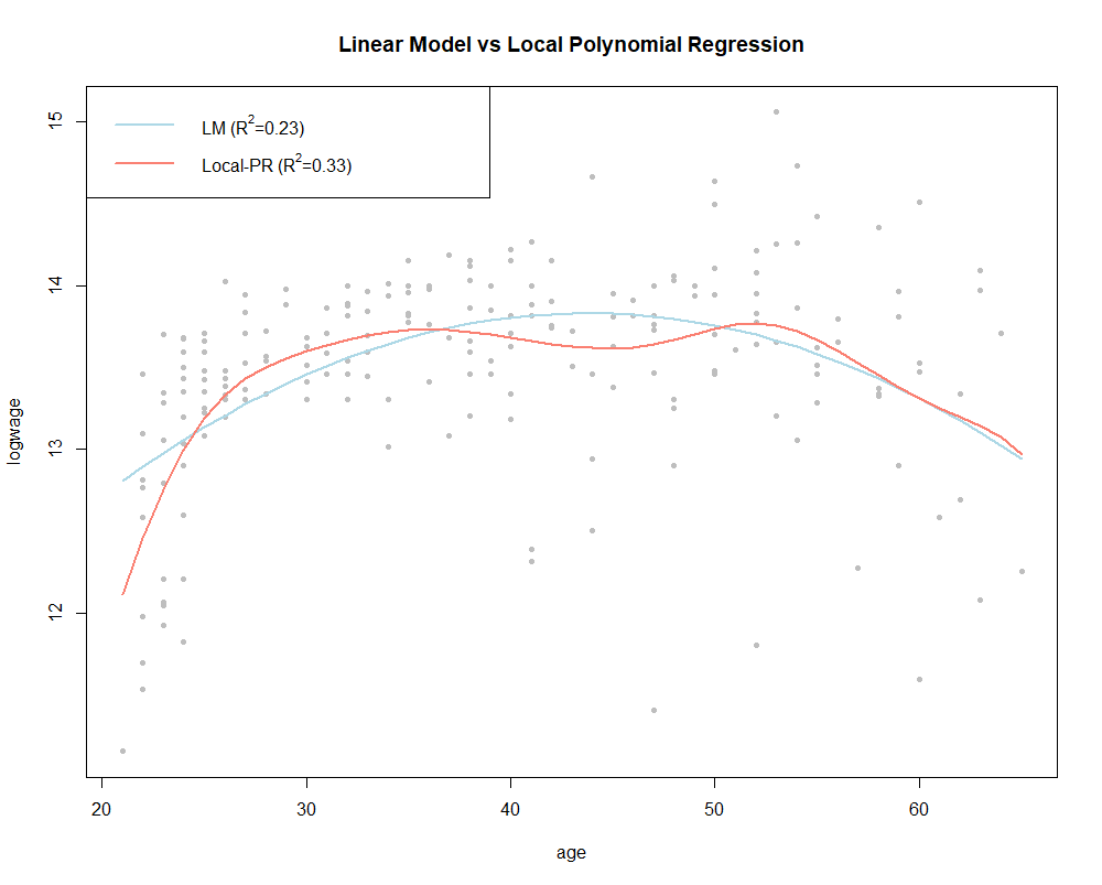

In Fig. 2 it is shown the parametric regression fit versus the non-parametric model.

For the non-parametric model, the bandwidth parameter is estimated by cross-validation using AIC criterion. Actually, in non-parametric modelling, as opposite to linear parametric models, often it is convenient to not to assume homoscedasticity and estimate the conditional variance. The following R code has been used to generate the presented example:

library(“np”)

data(“cps71”)

model.par <- lm(logwage ~ age + I(age^2), data = cps71)

summary(model.par)

model.np <- npreg(logwage ~ age, regtype = “ll”, bwmethod = “cv.aic”, gradients = TRUE, data = cps71)

summary(model.np)

plot(cps71$age, cps71$logwage, type=”o”, ylab=”logwage”, xlab=”age”, main=”Linear Model vs Local Polynomial Regression”)

lines(cps71$age, model.par$fitted.values, col=”lightblue”, lwd=2)

lines(cps71$age, fitted(model.np), col=”salmon”, lwd=2)

legend(“topleft”, legend = c(expression(paste(“LM (“, R^2, “=0.23)”)), expression(paste(“Local-PR (“, R^2, “=0.33)”))), col=c(“lightblue”, “salmon”), lwd=2)